Chapter 3

Random Networks

Code by : Abolfazl Ziaeemehr

• https://github.com/Ziaeemehr

# uncomment and run this line to install the package on colab
# !pip install "git+https://github.com/Ziaeemehr/netsci.git" -q

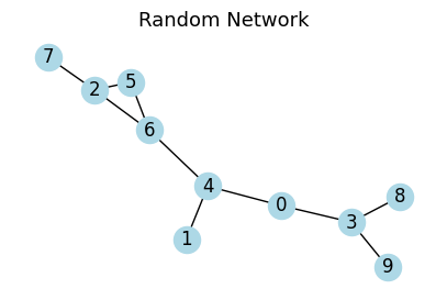
A random network consists of N nodes where each node pair is connected with probability p. To construct a random network we follow these steps:

1. Start with N isolated nodes.

2. Select a node pair and generate a random number between 0 and 1. If the number exceeds p, connect the selected node pair with a link, otherwise leave them disconnected.

3. Repeat step (2) for each of the N(N-1)/2 node pairs.

import random
import numpy as np
import networkx as nx
import seaborn as sns
import matplotlib.pyplot as plt
from netsci.plot import plot_graph

LABELSIZE = 13
plt.rc('axes', labelsize=LABELSIZE)
plt.rc('axes', titlesize=LABELSIZE)
plt.rc('figure', titlesize=LABELSIZE)
plt.rc('legend', fontsize=LABELSIZE)
plt.rc('xtick', labelsize=LABELSIZE)
plt.rc('ytick', labelsize=LABELSIZE)

def create_random_network(N, p):
    G = nx.Graph()  # Initialize an empty graph
    G.add_nodes_from(range(N))  # Add N isolated nodes

    # Iterate through each possible node pair
    for i in range(N):
        for j in range(i + 1, N):
            if random.random() <= p:  # Generate a random number and compare it with p
                G.add_edge(i, j)  # Connect the nodes if the condition is met

    return G

# Example usage:
N = 10  # Number of nodes
p = 0.3  # Probability of edge creation

seed=2
random.seed(seed)
np.random.seed(seed)

random_network = create_random_network(N, p)
plot_graph(random_network, seed=2, figsize=(5, 3), title="Random Network")

<Axes: title={'center': 'Random Network'}>

Other option would be to use the nx.gnp_random_graph function from NetworkX, which generates random graphs with a given number of nodes and a given probability of edge creation.

G = nx.gnp_random_graph(N, p)

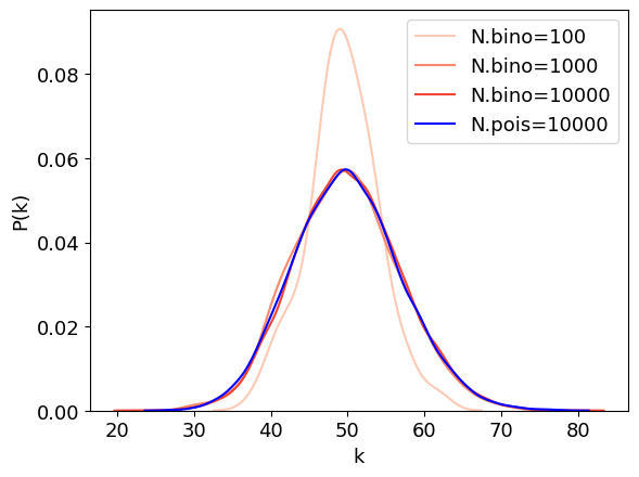
Binimial distribution

Degree distribution in a random network follows a binomial distribution.

# make a random graph with N nodes and average degree of k
np.random.seed(2)

num_nodes = [100, 1000, 10000]
average_degree = 50
lambd = 50
colors1 = plt.cm.Reds(np.linspace(0.2, 0.6, len(num_nodes)))

for i in range(len(num_nodes)):
    probability = average_degree / num_nodes[i]
    graph_b = nx.gnp_random_graph(num_nodes[i], probability)
    degrees = [d for n, d in graph_b.degree()]
    sns.kdeplot(degrees, fill=False, label=f"N.bino={num_nodes[i]}", color=colors1[i])

s = np.random.poisson(lambd, num_nodes[-1])
sns.kdeplot(s, fill=False, label=f"N.pois={num_nodes[i]}", color='b')

plt.xlabel("k")
plt.ylabel("P(k)")
plt.legend();

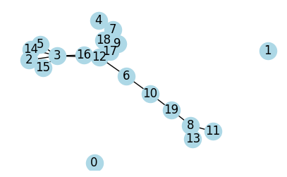
The evolution of a random network

import networkx as nx
import matplotlib.pyplot as plt

# Step 1: Generate a random graph (Erdős-Rényi model)
n = 20  # number of nodes
p = 0.12  # probability of edge creation
G = nx.erdos_renyi_graph(n, p)

# Step 2: Find all connected components
connected_components = list(nx.connected_components(G))

# Step 3: Calculate the size of each connected component
component_sizes = [len(component) for component in connected_components]

# Display the graph and component sizes
print("Connected Components:")
for i, component in enumerate(connected_components):
    print(f"Component {i + 1}: Size {len(component)}")

# Optionally, visualize the graph
plot_graph(G, seed=2, figsize=(5, 3));

Connected Components:
Component 1: Size 1
Component 2: Size 1
Component 3: Size 18

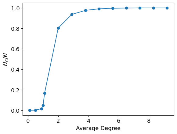
Plotting the size of giant connected component vs average degree

N = int(1e4)
print(f"N={N}, Ln(N)= {np.log(N)}")
k_avg = [.1, 0.5, 0.9, 1.0] + np.linspace(1.1, np.log(N), 10).tolist()
giant_component_sizes = []
for i in range(len(k_avg)):
    p = k_avg[i] / N
    G = nx.erdos_renyi_graph(N, p)
    connected_components = list(nx.connected_components(G))
    component_sizes = [len(component) for component in connected_components]
    giant_component_size = max(component_sizes)
    giant_component_sizes.append(giant_component_size)

    print(f"average k = {k_avg[i]:10.3f}, giant_component_size={giant_component_size:10d}")

giant_component_sizes = np.array(giant_component_sizes)/N
plt.plot(k_avg, giant_component_sizes, marker='o', label='Giant Component Size')
plt.xlabel(r'Average Degree')
plt.ylabel(r'$N_G / N$');

N=10000, Ln(N)= 9.210340371976182
average k =      0.100, giant_component_size=         4
average k =      0.500, giant_component_size=        11
average k =      0.900, giant_component_size=       164
average k =      1.000, giant_component_size=       480
average k =      1.100, giant_component_size=      1682
average k =      2.001, giant_component_size=      8028
average k =      2.902, giant_component_size=      9363
average k =      3.803, giant_component_size=      9755
average k =      4.705, giant_component_size=      9909
average k =      5.606, giant_component_size=      9967
average k =      6.507, giant_component_size=      9989
average k =      7.408, giant_component_size=      9999
average k =      8.309, giant_component_size=      9997
average k =      9.210, giant_component_size=      9998

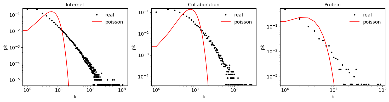
Degree distribution of real networks

from netsci.utils import load_sample_graph, list_sample_graphs
from netsci.analysis import graph_info

# on google colab:
nets = ['Collaboration', 'Internet', 'PowerGrid', 'Protein', 'PhoneCalls', 'Citation', 'Metabolic', 'Email', 'WWW', 'Actor']

# on local:
graphs = list_sample_graphs()
graphs.keys()

dict_keys(['Collaboration', 'Internet', 'PowerGrid', 'Protein', 'PhoneCalls', 'Citation', 'Metabolic', 'Email', 'WWW', 'Actor'])

On Google Colab only:

from google.colab import drive
import os

# URL of the zip file to be downloaded
url = "https://networksciencebook.com/translations/en/resources/networks.zip"
# Mount Google Drive
drive.mount('/content/drive')
# Create the 'network_science' directory in MyDrive if it doesn't exist
network_science_dir = '/content/drive/MyDrive/network_science'
os.makedirs(network_science_dir, exist_ok=True)
# empty the directory
!rm -rf /content/drive/MyDrive/network_science/*
# Change directory to 'network_science'
os.chdir(network_science_dir)
# Download the zip file to the 'network_science' directory
!wget $url -O networks.zip
# Unzip the downloaded file in the 'network_science' directory
!unzip networks.zip

json_file = "https://raw.githubusercontent.com/Ziaeemehr/netsci/main/netsci/datasets/sample_graphs.json"
# download json file
!wget $json_file -O sample_graphs.json

# on colab:
# G_collab = load_sample_graph('Collaboration', verbose=True, colab_path=network_science_dir)

# on local:
G_collab = load_sample_graph('Collaboration', verbose=True)
graph_info(G_collab)

Successfully loaded Collaboration
================================
Scientific collaboration network based on the arXiv preprint archive's
 Condense Matter Physics category covering the period from January 1993 to April 2003.
 Each node represents an author, and two nodes are connected if they co-authored at
 least one paper in the dataset. Ref: Leskovec, J., Kleinberg, J., & Faloutsos, C. (2007).
 Graph evolution: Densification and shrinking diameters.
 ACM Transactions on Knowledge Discovery from Data (TKDD), 1(1), 2.
Graph information
Directed                                :                False
Number of nodes                         :                23133
Number of edges                         :                93439
Average degree                          :               8.0784
Connectivity                            :         disconnected

Figure 3.6

from scipy.stats import poisson
from collections import Counter

fig, ax = plt.subplots(1,3, figsize=(15,4))

c = 0
for net in ["Internet", "Collaboration", "Protein"]:
    G = load_sample_graph(net) # on colab: add colab_path=network_science_dir
    degrees = [G.degree(n) for n in G.nodes()]
    degree_count = Counter(degrees)
    k, pk = zip(*degree_count.items())
    k = np.array(k)
    pk = np.array(pk)/sum(pk)


    ax[c].loglog(k, pk, 'k.', label='real')
    ax[c].set_xlabel("k")
    ax[c].set_ylabel("pk");
    ymin, ymax = np.min(pk)*0.9, np.max(pk)*1.1

    # add poisson distribution to graph

    k = np.arange(0, max(degrees)+1)
    pk_poisson = poisson.pmf(k, np.mean(degrees))
    ax[c].loglog(k, pk_poisson, 'r', label='poisson')
    # plt.ylim([1e-5, 1])
    ax[c].legend(frameon=False);
    ax[c].set_ylim([ymin, ymax])
    ax[c].set_title(net)
    c += 1

plt.tight_layout()

Clustering coefficient

The local clustering coefficient of a random network is

\[C_i = p= \frac{⟨k⟩}{N}\]

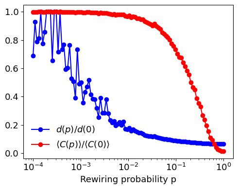
To analyze the dependence of the average path length \(d(p)\) and the clustering coefficient \(\langle C(p) \rangle\) on the rewiring parameter \(p\) for a small-world network, you can use the Watts-Strogatz model. This model begins with a regular lattice and introduces randomness by rewiring each edge with probability \(p\). Here’s a step-by-step guide on how to perform this analysis:

1. Generate a regular lattice: Create a regular ring lattice with \(N\) nodes where each node is connected to its \(k\) nearest neighbors.

2. Rewire edges: For each edge in the lattice, rewire it with probability \(p\). This involves replacing the existing edge with a new edge that connects the node to a randomly chosen node in the network.

3. Compute :math:`d(p)` and :math:`langle C(p) rangle`:

   • \(d(p)\) is the average shortest path length between all pairs of nodes in the network.

   • \(\langle C(p) \rangle\) is the average clustering coefficient of all nodes in the network.

4. Normalize by :math:`d(0)` and :math:`langle C(0) rangle`:

   • \(d(0)\) is the average path length of the regular lattice (when \(p=0\)).

   • \(\langle C(0) \rangle\) is the average clustering coefficient of the regular lattice (when \(p=0\)).

5. Plot the results: Plot \(d(p)/d(0)\) and \(\langle C(p) \rangle / \langle C(0) \rangle\) as functions of \(p\) on a log scale to observe the small-world phenomenon.

import numpy as np
import networkx as nx
import matplotlib.pyplot as plt

# Parameters
N = 1000  # Number of nodes
k = 10    # Each node is connected to k nearest neighbors in ring topology
p_values = np.logspace(-4, 0, num=100)  # Rewiring probabilities

# Initialize lists to store results
average_path_lengths = []
clustering_coefficients = []

# Generate the initial regular lattice
G0 = nx.watts_strogatz_graph(N, k, 0)
d0 = nx.average_shortest_path_length(G0)
C0 = nx.average_clustering(G0)

for p in p_values:
    G = nx.watts_strogatz_graph(N, k, p)
    d = nx.average_shortest_path_length(G)
    C = nx.average_clustering(G)
    average_path_lengths.append(d / d0)
    clustering_coefficients.append(C / C0)

# Plotting
plt.figure(figsize=(5, 4))

# Average path length plot
plt.plot(p_values, average_path_lengths, marker='o', linestyle='-', color='blue', label=r"$d(p)/d(0)$")

# Clustering coefficient plot
plt.plot(p_values, clustering_coefficients, marker='o', linestyle='-', color='red', label=r"$\langle C(p) \rangle / \langle C(0) \rangle$")
plt.xscale('log')
plt.xlabel('Rewiring probability p')
plt.legend(frameon=False)
plt.tight_layout()
plt.show()