Chapter 3

Two-dimensional systems and state space

Code by : Abolfazl Ziaeemehr - https://github.com/Ziaeemehr

# uncomment and run this line to install the package on colab
# !pip install "git+https://github.com/Ziaeemehr/spikes.git" -q

import sympy as sp
import numpy as np
from sympy import lambdify
import matplotlib.pyplot as plt
from scipy.linalg import eig, inv
from scipy.integrate import odeint
from IPython.display import display, Math
from spikes.solver import solve_linear_system_numerical

Analytical Solution for \(\frac{d\vec{X}}{dt} = A\vec{X} + \vec{B}\)

Let’s derive the analytical solution step-by-step for the differential equation \(\frac{d\vec{X}}{dt} = A\vec{X} + \vec{B}\), assuming \(\lambda_1 \neq \lambda_2\).

Steps to Solve Analytically

1. Find the Equilibrium State The equilibrium state \(\vec{X}_{eq}\) is given by:

   \[\vec{X}_{eq} = -A^{-1} \vec{B}\]

2. Determine the Eigenvalues and Eigenvectors The eigenvalues \(\lambda_1\) and \(\lambda_2\) are solutions to the characteristic equation:

   \[\det(A - \lambda I) = 0\]

   where \(I\) is the identity matrix.

Let’s denote the eigenvectors corresponding to \(\lambda_1\) and \(\lambda_2\) as \(\vec{v}_1\) and \(\vec{v}_2\), respectively.

3. General Solution The general solution for the system \(\frac{d\vec{X}}{dt} = A\vec{X}\) can be written as:

   \[\vec{X}(t) = c_1 \vec{v}_1 e^{\lambda_1 t} + c_2 \vec{v}_2 e^{\lambda_2 t}\]

   where \(c_1\) and \(c_2\) are constants determined by initial conditions.

4. Incorporate the Equilibrium State To incorporate \(\vec{B}\), we use the transformation \(\vec{X} = \vec{X}_{hom} + \vec{X}_{eq}\), where \(\vec{X}_{hom}\) is the homogeneous solution. Thus:

   \[\vec{X}(t) = \vec{X}_{hom}(t) + \vec{X}_{eq}\]
   \[\vec{X}(t) = c_1 \vec{v}_1 e^{\lambda_1 t} + c_2 \vec{v}_2 e^{\lambda_2 t} + \vec{X}_{eq}\]

This gives us the analytical solution in the form:

\[\begin{split}\vec{X}(t) = \begin{pmatrix} a_1 e^{\lambda_1 t} + a_2 e^{\lambda_2 t} \\ b_1 e^{\lambda_1 t} + b_2 e^{\lambda_2 t} \end{pmatrix} + \vec{X}_{eq}\end{split}\]

5. General Solution for Repeated Eigenvalues

The general solution when \(\lambda_1 = \lambda_2 = \lambda\) is:

\[\vec{X}(t) = (c_1 + c_2 t) e^{\lambda t} \vec{v} + \vec{X}_{eq}\]

solve_linear_system_numerical??

Signature: solve_linear_system_numerical(A, B, X0, t)
Source:
def solve_linear_system_numerical(A, B, X0, t):
    """
    Solves the differential equation dX/dt = AX + B.

    Parameters:
    A (numpy.ndarray): Coefficient matrix.
    B (numpy.ndarray): Constant vector.
    X0 (numpy.ndarray): Initial condition vector.
    t (numpy.ndarray): Array of time points at which to solve.

    Returns:
    numpy.ndarray: Array of solution vectors at each time point.
    """
    # Equilibrium state
    X_eq = -inv(A) @ B

    # Eigenvalues and eigenvectors
    eigenvalues, eigenvectors = eig(A)

    # Solve for the constants a1, a2, b1, b2
    def system(X, t):
        return A @ X + B

    sol = odeint(system, X0, t)

    return {"x": sol, "xeq": X_eq, "ev": eigenvalues, "evec": eigenvectors}
File:      ~/git/workshops/spikes/spikes/solver.py
Type:      function

Numerical solution

B_np = np.array([7, 1])
X0_np = np.array([0, 0])
A_np = np.array([[-9, -5], [1, -3]])
t_range = np.linspace(0, 3, 100)
solution_num = solve_linear_system_numerical(
    A_np, B_np, X0_np, t_range
)
solution_num["x"].shape

(100, 2)

Analytical solution

t = sp.Symbol('t')
x1, x2 = sp.Function('x1')(t), sp.Function('x2')(t)
A = sp.Matrix(A_np)
X = sp.Matrix([x1, x2])
B = sp.Matrix(B_np)
X0 = sp.Matrix(X0_np)

dx_dt = A * X + B
system = [sp.Eq(sp.diff(x1, t), dx_dt[0]), sp.Eq(sp.diff(x2, t), dx_dt[1])]
sol_hom = sp.dsolve(system)

t0 = 0
constants = sp.solve(
    [sol.rhs.subs(t, t0) - x0 for sol, x0 in zip(sol_hom, X0)]
)

sol_hom_constants = [sol.rhs.subs(constants) for sol in sol_hom]
final_solution = [sol_hom for sol_hom in sol_hom_constants]

# display solutions
for i, sol in enumerate(final_solution, 1):
    display(Math(f'x_{i}(t) = {sp.latex(sol)}'))

# evaluate solution
x_functions = [lambdify((t,), sol, "numpy") for sol in final_solution]
x_values = [x_func(t_range) for x_func in x_functions]

# plot solutions
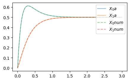
plt.figure(figsize=(5,3))
for i in range(2):
    plt.plot(t_range, x_values[i], label=f'$X_{i} a$', alpha=0.5)

# plot numerical solution to compare
for i in range(2):
    plt.plot(t_range, solution_num['x'][:, i], label=f'$X_{i} num$', ls='--', alpha=0.5)

plt.legend(loc='upper right');
print("Equilibrium state:", solution_num['xeq'])
print("Eigenvalues:", solution_num['ev'])

$\displaystyle x_1(t) = \frac{1}{2} + \frac{3 e^{- 4 t}}{4} - \frac{5 e^{- 8 t}}{4}$

$\displaystyle x_2(t) = \frac{1}{2} - \frac{3 e^{- 4 t}}{4} + \frac{e^{- 8 t}}{4}$

Equilibrium state: [0.5 0.5]
Eigenvalues: [-8.+0.j -4.+0.j]

We can define the above process as a function solve_system_of_equations that takes in the coefficient matrix A (any size) , rhs of B and initial conditions X0 and time range t_range. The function will return the final analytical solution and evalution of the function at fiven time interval.

from spikes.solver import solve_system_of_equations

B_np = np.array([7, 1])
X0_np = np.array([0, 0])
A_np = np.array([[-9, -5], [1, -3]])
t_range = np.linspace(0, 3, 100)
solution_num = solve_linear_system_numerical(
    A_np, B_np, X0_np, t_range
)
solution_num["x"].shape

final_solution, x_values = solve_system_of_equations(A_np, B_np, X0_np, t_range)
for i, sol in enumerate(final_solution, 1):
    display(Math(f'x_{i}(t) = {sp.latex(sol)}'))

# plot solutions
plt.figure(figsize=(5,3))
for i in range(2):
    plt.plot(t_range, x_values[i], label=f'$X_{i} a$', alpha=0.5)

# plot numerical solution to compare
for i in range(2):
    plt.plot(t_range, solution_num['x'][:, i], label=f'$X_{i} num$', ls='--', alpha=0.5)

plt.legend(loc='upper right');
print("Equilibrium state:", solution_num['xeq'])
print("Eigenvalues:", solution_num['ev'])

$\displaystyle x_1(t) = \frac{1}{2} + \frac{3 e^{- 4 t}}{4} - \frac{5 e^{- 8 t}}{4}$

$\displaystyle x_2(t) = \frac{1}{2} - \frac{3 e^{- 4 t}}{4} + \frac{e^{- 8 t}}{4}$

Equilibrium state: [0.5 0.5]
Eigenvalues: [-8.+0.j -4.+0.j]

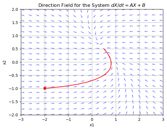
Direction Fields

from spikes.plot import plot_direction_field
plot_direction_field?

Signature:
plot_direction_field(
    A: numpy.ndarray,
    B: numpy.ndarray,
    x1_range: tuple = (-2, 2),
    x2_range: tuple = (-2, 2),
    num_points: int = 20,
    ax=None,
    xlabel: str = 'x1',
    ylabel: str = 'x2',
    title: str = 'Direction Field for the System $dX/dt = AX + B$',
    **kwargs,
)
Docstring:
Plots the direction field for the system dx/dt = A * X + B.

Parameters:
- A: 2x2 numpy array, the coefficient matrix for the linear system.
- B: 1x2 numpy array, the constant vector.
- x1_range: tuple, the range for x1 values (default: (-10, 10)).
- x2_range: tuple, the range for x2 values (default: (-10, 10)).
- num_points: int, the number of points per axis in the grid (default: 20).
File:      ~/git/workshops/spikes/spikes/plot.py
Type:      function

from spikes.plot import plot_direction_field

ax = plot_direction_field(A_np, B_np, x1_range=(-3,3), alpha=.5, color="b")

#plot a solution trajectory
x0 = np.array([-2, -1])
sol = solve_linear_system_numerical(A_np, B_np, x0, t_range)['x']
ax.plot(sol[:, 0], sol[:, 1], 'r-')
circle = plt.Circle(x0, 0.1, color='r', fill=False)
ax.plot(x0[0], x0[1], 'ro');